Modelling the Relationship Between Merchandise Trade Flows and Some Macroeconomic Variables in Ghana

Azebre Abu Ibrahim; Anuwoje Ida Logubayom Abonongo

doi:doi:10.11648/j.ajtas.20241305.15

Research Article |

| Peer-Reviewed

Modelling the Relationship Between Merchandise Trade Flows and Some Macroeconomic Variables in Ghana

Azebre Abu Ibrahim^*

, Anuwoje Ida Logubayom Abonongo

Published in American Journal of Theoretical and Applied Statistics (Volume 13, Issue 5)

Received: 2 September 2024 Accepted: 25 September 2024 Published: 29 October 2024

Views: Downloads:

Download PDF

Share This Article

Twitter
Linked In
Facebook

Abstract

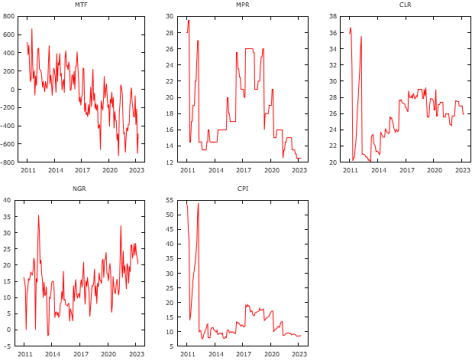
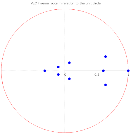
Macroeconomic variables serve as economic indicators that offer valuable insights into the overall health and stability of an economy. Changes in these variables can have significant impacts on a country's trade balance and overall economic performance. This study employed multivariate time series analysis to study the relationship between Merchandise Trade Flows (MTF), Monetary Policy Rate (MPR), Commercial Lending Rate (CLR), Nominal Growth Rate (NGR) and Consumer Price Index (CPI) with Money Supply (MoS) as exogenous variable. The nature of trend in each series was investigated. The results revealed that quadratic trend model best models MTF, MPR, CLR and NGR whiles an exponential trend best models CPI. Johansen’s co-integration test with unrestricted trend performed revealed the existence of long-run equilibrium relationships between the variables and three (3) co-integrating equations described this long-run relationship. In terms of short-run relationships, the VEC (2) model revealed that, CLR, NGR, MoS have positive and significant impact on MTF. CLR, NGR and MoS have positive and significant impact on MPR, NGR have positive and significant impact on CLR, CPI and MoS have significant impact on NGR whiles NGR and MoS have significant impact on CPI. Model diagnostics performed on the VEC (2) model showed that, all the model parameters are structurally stable over time and the residuals of the individual models are free from serial correlation and conditional heteroscedasticity. Forecast error variance decomposition (FEVD) analysis showed that each variable primarily explained its own variance and the influence of other variables increase over time. Hence, adopting a broad perspective on macroeconomic variables can help policymakers anticipate and mitigate ripple effects across various economic sectors.

Published in	American Journal of Theoretical and Applied Statistics (Volume 13, Issue 5)
DOI	10.11648/j.ajtas.20241305.15
Page(s)	157-174
Creative Commons	This is an Open Access article, distributed under the terms of the Creative Commons Attribution 4.0 International License (http://creativecommons.org/licenses/by/4.0/), which permits unrestricted use, distribution and reproduction in any medium or format, provided the original work is properly cited.
Copyright	Copyright © The Author(s), 2024. Published by Science Publishing Group

Keywords

Macroeconomic Variables, Merchandise Trade Flows, Co-Integration

1. Introduction

The role of international trade and various economic variables significantly impacts the growth and development of countries

[3, 25]

. International trade promotes growth by expanding markets, allocating resources efficiently, and driving innovation, offering countries access to wider consumer bases, enhancing productivity, and promoting the quality of goods and services. It also facilitates technological transfer, foreign direct investment, industrial development, and employment opportunities.

International trade, which includes exports and imports, is encouraged by most governments as a driver of economic progress

[17]

. However, many governments take steps to limit imports and focus on increasing exports by seeking foreign market expansion

[14]

. Merchandise trade enables countries to obtain goods and resources that may not be available domestically and specialize in producing goods where they have a comparative advantage, leading to increased efficiency and economic growth. Ghana aims to diversify its exports and imports, attract foreign direct investment, and create employment opportunities. However, Ghana's ability to compete in international trade has decreased in the past decade

[22]

, and it faces higher trading costs with most African partners

[18]

Other macroeconomic variables like monetary policy rates, inflation, exchange rates, and interest rates also influence the overall economy

[1, 9, 12, 15]

. These variables collectively affect economic growth, inflation, and exchange rates.

Although various studies

[11-13, 15]

have explored merchandise trade flows, monetary policy, interest rates, inflation, exchange rates, and their impacts on different economic variables, there is a need for a holistic understanding of how these economic variables interact among themselves in Ghana's economic context. The existing literature highlights a need for further research concerning merchandise trade flows and their interactions with other economic variables in Ghana

[3, 16, 17, 21, 24, 25]

This study provides empirical evidence on both short-run and long-run dynamics, demonstrating how changes in key economic indicators such as the MPR, CLR, NGR, CPI and MTF influences each other. By utilizing multivariate time series models and monthly data from Bank of Ghana, the study offers a detailed analysis of the interconnections, and co-integration among these variables. This comprehensive approach highlights the importance of considering multiple economic factors simultaneously to understand the macroeconomic dynamics in Ghana. Given the significant role that trade and other macroeconomic factors in the country's economy, comprehending these relationships can inform better policy-making. The study aims to provide insights that can help stabilize and improve Ghana’s economic performance. Additionally, understanding forecast uncertainties can aid in creating more resilient economic policies. Finally, the goal is to equip policymakers with the knowledge needed to make informed decisions that can enhance economic stability and growth in the country.

2. Review of Literature

Global trade flows and economic variables are shaped by a myriad of interconnected factors, presenting a complex landscape that researchers have extensively explored in recent years. For instance, the gravity model was utilized to dissect international trade flows

[24]

. The findings highlighted the significant impact of geographical location, economies of scale, and trade system arrangements on trade flows. China's agricultural trade was found to be closely tied to the GDP size of its trading partners and the distance between them. However, demographic factors and exchange rates showed negligible influence

[24]

The volatility of international trade flows and its correlation with economic growth was explored

[7]

. The study uncovered that trade volatility is affected by common factors across all nations, country-specific elements, and changes in trading partner characteristics. Trade diversification emerged as a strategy to mitigate volatility, especially for developing economies

[7]

Stašys and Tananaiko focused on the impact of tariff and non-tariff measures on global trade dynamics

[20]

. They noted that while free trade agreements bolster trading flows by removing barriers, tariffs continue to wield significant influence. Additionally, recent studies shed light on evolving factors like tariff reductions, technological advancements, shifts from protectionism to free trade ideologies, and Africa's growing role in the global economy, all of which contribute to trade imbalances in specific regions

[16]

The role of natural resources in trade dynamics was explored

[19]

. The study observed that liberalized trade policies increase resource exports but improvements in resource efficiency can decrease exports. Environmental policies like energy and resource taxes also shape resource trade dynamics significantly

[19]

Moving beyond trade, monetary policy's pivotal role in shaping economic conditions was emphasized

[1]

. The study highlighted how central banks' policy rates influence interest rates, investment, borrowing costs, and consequently, global trade flows. Inflation, another critical economic variable, impacts consumer purchasing power, export competitiveness, and the cost dynamics of imports and exports

[2, 12]

Furthermore, more studies provided insights into the role of foreign direct investment (FDI), infrastructure, trade policies, geographical factors, and internal considerations in shaping trade patterns

[3-5, 25]

Comparative studies by

[9]

explored the implications of different financial market structures on macroeconomic variables. The study found that international financial market structures significantly impact economic outcomes like growth rates, inflation, interest rate parity, and exchange rates. Similarly, studies on Ethiopia's coffee exports, Nigeria's trade patterns, Pakistan's bilateral trade performance, and Indonesia's trade balance shed light on the diverse factors influencing trade dynamics, from geopolitical factors to economic policies and market conditions.

Various global perspectives shed light on Ghana's trade flows, revealing insights crucial for understanding its economic dynamics

[23]

. International organizations like the World Bank and World Trade Organization (WTO) contribute significantly to this discourse. In 2022, the World Bank conducted a trade competitiveness diagnostics aimed at enhancing Ghana's trade performance within the African Continental Free Trade Area (AfCFTA). Their research provided policy recommendations to strengthen Ghana's trade competitiveness, emphasizing the importance of strategic measures in navigating the global market.

Yeboah, E. researched into foreign direct investment (FDI) in Ghana, showcasing the distribution of FDI across sectors and regions

[25]

. This analysis offered a global perspective on the industries attracting substantial investment, thus highlighting sectors pivotal to Ghana's trade flows. Additionally, a study explored the determinants of FDI in Ghana, aiding in understanding the factors shaping the country's trade patterns

[3]

Examining regional and continental engagements is crucial for comprehensively understanding Ghana's trade and economic dynamics. Raga provided a macroeconomic and trade profile of Ghana, discussing opportunities and challenges in implementing the AfCFTA

[18]

. This broader perspective underscores Ghana's potential to strengthen trade connections within Africa and globally.

Methodological approaches in existing literature further enrich the understanding of Ghana's economic landscape. Econometric techniques like system models allow for rigorous analysis of economic relationships, such as the impact of monetary policy on interest and inflation rates

[1]

. Gravity models used to research on Ghana's trade within ECOWAS, offer quantitative insights into trade determinants considering economic variables and geographic proximity

[21]

. Panel regression analysis, utilized in investigating South Africa's fruit exports to West Africa, helps identify influential trade factors across entities and time

[17]

. Statistical models (regression models, fixed and random effects models, Granger causality test, impulse response function, and so on) are being used in the analysis of exchange rate volatility in Pakistan, reveal relationships between economic variables

[2]

. Advancements in econometric techniques, including instrumental variable regression, dynamic panel models, vector autoregressive (VAR) models, co-integration, vector error correction (VEC) models, autoregressive distributed lag (ARDL) models and general autoregressive conditional heteroscedasticity (GARCH) models, offer promising avenues to capture the dynamic complexities and interplay between economic variables. These methodological innovations further enrich the understanding of Ghana's economic dynamics on a global scale.

Further research in modeling the relationship between merchandise trade flows and some macroeconomic variables in Ghana is imperative despite existing literature. This necessity arises due to the evolving nature of global economic dynamics and Ghana's economic landscape, requiring a continually deeper understanding of the interconnectedness between multiple macroeconomic factors. Additional research can offer more comprehensive insights, address methodological limitations, and provide timely and most recent data to guide effective policy formulation to encourage Ghana's economic growth and foster sustainable economic development.

Multivariate time series models are ideal for researching the relationship between merchandise trade flows and macroeconomic variables in Ghana due to their ability to capture complex interactions, dynamic changes over time, identify causal relationships, provide forecasting capabilities, and offer statistical rigor, all of which are crucial for gaining thorough insights into Ghana's economic landscape

[22, 23]

3. Methods of Data Analysis

The study used multivariate time series models such as co-integration analysis, vector error correction (VEC) model, impulse response function analysis (IRF) and forecast error variance decomposition (FEVD) analysis for the data. This allows for a robust and comprehensive analysis by capturing different aspects, nuances, and potential short-run and long-run relationships within the data.

3.1. Source of Data

The study utilized monthly time series data on each variable from the Bank of Ghana website. The data span from January, 2011 to April, 2023.

3.2. Trend Models

Trend analysis helps to identify and understand the underlying patterns and directions of the data over the specified period. It also helps in detecting and accounting for non-stationarity, which is essential for accurate model specification and reliable statistical inference. Identifying the trend in the variables considered is also essential, so as to identify the form of co-integration analysis to perform (either with restricted trend or unrestricted trend). If the variables exhibit quadratic trends, then the co-integration analysis will be done with unrestricted trend and vice versa. Three trend models were considered: thus the linear, quadratic and exponential trend models as given in equations 1, 2 and 3 respectively.

Y_{t} = β_{0} + β_{1} t + ε_{t},

(1)

Y_{t} = β_{0} + β_{1} t + β_{2} t^{2} + ε_{t},

.(2)

Y_{t} = β_{0} + (β_{1} ᵗ) + ε_{t}

,(3)

where

β_{0}

is the intercept,

β_{1} and β_{2}

are the coefficients,

t

is the value of time unit, and

ε_{t}

is the error term.

3.3. Unit Root Test (Test for Stationarity)

In time series analysis, it is essential to investigate the presence or otherwards of unit root in a series. The presence or absence of unit roots helps to identify the nature of the processes that generates the time series data and to investigate the order of integration (number of time series is differenced to achieve stationarity) of a series which gives a guide the appropriate time series model for the data and to prevent spurious results. A variable is said to be covariance or weakly stationary if its mean, variance and the autocovariance are finite and time invariant.

Accurate identification of integration order guides proper model specification, avoiding biased parameter estimates and unreliable forecasts. The study use Augmented Dickey Fuller (ADF) test to investigate presence of unit roots in the variables.

The ADF is an extension of the Dickey-Fuller test. With the Dickey-Fuller test, the null hypothesis (H₀):

α = 1

which implied the time series contains unit roots uses the regression model given as

y_{t} = β + β_{t} + {αy}_{t - 1} + \emptyset ∆ y_{t - 1} + ε_{t}

(4)

where

y_{t - 1}

is lag 1 of the series and

∆ y_{t - 1}

is the first difference of the series at time

t - 1

The test statistic for ADF test is given in equation 5.

ADF = \frac{Ŷ}{SE (Ŷ)}

(5)

where

Ŷ

is the least square coefficient and

SE (Ŷ)

is the standard error of

Ŷ

The null hypothesis is rejected if the p-value associated with the ADF statistic is less than the chosen significance level (0.05).

3.4. Lag Order Selection for Co-Integration and Vec Model

In co-integration and VEC model estimation, selecting the appropriate lag order is crucial. This involves determining the optimal number of lagged for the co-integration analysis and fitting the VEC model. The optimum lag terms in the model can be identified using model selection criteria like Akaike Information Criterion (AIC), Schwarz Bayesian Information Criterion (SBIC), Hannan-Quinn Information criteria (HQIC) and likelihood ratio tests (LL). The aim is to strike a balance between model complexity and goodness of fit to accurately represent dynamic data relationships.

The test statistic for AIC, SBIC and HQIC are given in equations 6, 7 and 8 respectively.

AIC = - 2 In (L) + 2 k,

(6)

SBIC = - 2 In (L) + k In (N),

(7)

HQIC = - 2 In (L) + 2 k In (In (N)),

(8)

where

k

is the number of parameters in the model,

L

is the likelihood,

N

is the number of observations and

In

is the natural logarithm. The best lag order is selected by considering the lag with the lowest values of AIC, SBIC and HQIC values.

3.5. Testing for Co-Integration

Co-integration denotes a long-run equilibrium relationship between non-stationary time series variables over time. Co-integration is crucial in macroeconomic analysis because it helps identify the enduring equilibrium connection between variables and reveals their interdependencies over long time. It also gives ideas on how shocks in any of the economic variables affects the equilibrium relationship. The study primarily employed the Johansen test for co-integration to investigate the long-run relationship between the economic variables.

The Johansen co-integration test is based on the idea that if there is a co-integrating relationship among a set of variables, they will move together in the long run, even if they exhibit short-run fluctuations. The general Johansen co-integration tests the null hypothesis of no co-integration

(r = 0)

against the alternative hypothesis of co-integration

(r > 0)

. The rank of co-integration

(r)

is determined by the number of eigenvalues that are significantly different from zero. The number of statistically significant eigenvalues provides an estimate of the number of co-integrating relationships among the variables

[6, 8]

The Johansen test computes the race statistics (

λ_{trace})

and maximum eigenvalue statistics (

λ_{\max})

based on the estimated model. These statistics follow a chi-square (

χ^{2})

distribution. The decision criterion is, if the

λ_{trace}

λ_{\max}

exceeds the critical value at a specific significance level, the null hypothesis is rejected, suggesting the presence of co-integration.

The

λ_{trace}

and

λ_{\max}

statistics for Johansen co-integration are given in equation 9 and 10 respectively;

λ_{trace} (r) = - T \sum_{i = r + 1}^{g} In (1 - {\hat{λ}}_{i}),

(9)

and

λ_{\max} (r, r + 1) = - T In (1 - {\hat{λ}}_{r - 1})

(10)

where r is the number of co-integrating vectors (co-integration rank) under the null hypothesis and

λ_{i}

is the estimated value for the i^th ordered eigenvalue from the co-integrating vector and

T

is the number of observations.

The

λ_{trace}

is a joint test with the hypothesis:

H_{0} : rank (co - integration) \leq r (at most r integrated vector)

against

H_{1} : rank (co - integration) > r (at least r + 1 integrated vector)

The

λ_{\max}

conducts a different test on individual eigenvalues, and its null hypothesis is that the number of co-integrating vectors is r against the alternative of

r + 1 .

The hypothesis under the

λ_{\max}

are given as;

H_{0} : r = 0 versus H_{1} : 0 < r \leq g

H_{0} : r = 1 versus : 1 < r \leq g

H_{0} : r = 2 versus H_{1} : 2 < r \leq g

H_{0} : r = g - 1 versus H_{1} : r = g

Depending on the nature of trend in the endogenous variables in the study, the co-integration test can be performed with restricted trend or unrestricted trend. With unrestricted trend, there are quadratic trends in the levels of the variables and that the co-integrating equations are trend stationary. For a restricted trend, we assume linear trend in the levels of the series.

The null hypothesis of the Johansen’s test is rejected if the p-value associated with each test statistic is less than the significant level selected.

3.6. Vector Error Correction (VEC) Model

A VEC model is a specialized form of a Vector Autoregressive (VAR) model designed for non-stationary series known to be co-integrated. The VEC model is used in this study to investigate short run relationship between the endogenous variables. The VEC model incorporates co-integration restrictions into its specification, allowing for long-run convergence to the co-integrating relationships while permitting various short-run dynamics.

In a compact form, the VEC model helps to examine the short-run dynamics as well as the long-run equilibrium relationship (captured by the error correction term). The compact form of VEC (p) model is written in equation 12;

∆ y_{t} = β_{0} + \prod y_{t - 1} + Г_{1} ∆ y_{t - 1} + \dots + Г_{p - 1} ∆ y_{t - p + 1} + γ (\prod y_{t - 1} - β_{0}) + ε_{t},

(11)

where

∆ y_{t}

represents the first difference of the variables

(y_{t} - y_{t - 1})

β_{0}

is the constant term (intercept), Π is a

n \times n

matrix of coefficients for the lagged levels of

y_{t - 1}

{_{1} {, \dots, }_{P - 1}}_{}

are

n \times n

matrices of coefficients for the lagged first differences of

y_{t - i}

and

ε_{t}

is the error term.

The error correction term (ECT) is given by;

{ECT}_{t - 1} = γ (\prod y_{t - 1} - β_{0}),

(12)

where

{ECT}_{t - 1}

represents the error correction term at time,

t - 1

and

γ

is the adjustment coefficient. The error correction term (ECT) in the VEC model captures the adjustment process towards the long-run equilibrium, gradually correcting deviations from it through partial short-run adjustments.

3.7. Model Stability Test Using the Unit Circle

Statistical inference using a VEC (p) model rest significantly on the stability of its parameters over time. A stable VEC (p) process generates stationary time series with time invariant means, variances and covariance structure. The companion matrix of the VEC (p) process with p-endogenous variables and r co-integrating vectors (equations) has

p - r

unit eigenvalues; the process is stable if the moduli of the remaining eigenvalues are strictly less than one (1). The unit circle is use to assess the behavior of the estimated roots of the characteristic polynomial of the model. Each root of the characteristic polynomial corresponds to a lagged value of the variables in the model. When all roots are inside the unit circle (less than one (1), it indicates that the model is stable and vice versa.

The stability of the VEC (p) model enables us to write the VEC (p) process as an invertible moving average process from which further inference such as Impulse Response Analysis can be made. For a stable VEC (p) process, the effects of any deviations from long-run equilibrium gradually diminish over time, ensuring that the system does not exhibit explosive behavior.

3.8. The VEC Model Diagnostics

To use the VEC(p) for statistical inference, it is important to investigate whether/not the model adequately fit the series. This involves examining if the residuals are white noise series; thus whether they are free from serial correlation and conditional heteroscedasticity (non-constant variance). The ARCH-LM and Ljung-Box tests are used as diagnostic tools to assess the adequacy of the VEC model and to detect the presence of or otherwise of ARCH effects and serial correlation (autocorrelation) in the residuals of the fitted model respectively.

The Autoregressive Conditional Heteroscedasticity Lagrange Multiplier (ARCH-LM) test is conducted to assess whether there is evidence of heteroscedasticity in the residuals of the fitted model. The ARCH-LM test statistic is given as,

LM = n R^{2}

(13)

where

n

is the number of observations and

R^{2}

is the coefficient of determination of the axillary residual regression. The ARCH-LM test checks the null hypothesis that the variance of the residuals is homoscedastic (constant) against the alternative hypothesis that the variance is heteroscedastic.

The Ljung-Box test is used to tests for the presence of residual autocorrelation and residual independence. This test assesses whether there are significant serial correlations in the residuals beyond a certain lag. A rejection of the null hypothesis suggests the presence of residual autocorrelation. It involves regressing the residuals on lagged residuals and conducting a Ljung-Box test for residual autocorrelation. It tests the null hypothesis that there is no autocorrelation up to a certain lag order.

The test statistic for the Ljung-Box test is given in equation 14,

Q_{m} = T (T + 2) \sum_{k = 1}^{m} {(T - K)}^{- 1} r_{k}^{2}

,(14)

where

r_{k}^{2}

is the residual autocorrelation at lag

k

T

is the number of residuals,

m

is the number of times lags included in the test

Both the ARCH-LM and Ljung Box test are chi-square distributed. If the test statistic exceeds the critical value from the chi-square table (or p-value < 0.05), the null hypothesis in each case is rejected or if the p-value associated with each test is smaller than the critical values, the null hypothesis is rejected.

3.9. Impulse Response Function Analysis

Impulse response function (IRF) analysis is used to examines the response of each endogenous variable to a shock (sudden change) in the other variables in a stable VAR/VEC model

[10]

. The IRF analysis allows the study to assess the significance and persistence of the impact of shocks in the variables on each other. The test statistic for IRF is calculated based on the estimation of the VEC model and the variance-covariance matrix of the coefficients. The IRF analysis is typically used for hypothesis testing regarding the impact of shocks on variables in the system over time. The test statistic for IRF analysis is based on the Wald test, which evaluates the significance of the impulse responses. The Wald test statistic is computed using equation 15

Wald Test statistic = \frac{{IRF}_{t}}{SE ({IRF}_{T})},

(15)

where

{IRF}_{t}

is the impulse response coefficient at time

t

and

{SE (IRF}_{T})

is the standard error of the impulse response coefficient at time

t

When the impulse response coefficient at time

t

is equal to zero (that is,

{IRF}_{t} = 0)

, it indicates that there is no significant impact of the shock on the variable at that specific time point. Alternatively, when impulse response coefficient at time t is not equal to zero (that is,

{IRF}_{t} \neq 0)

, it shows a significant impact of the shock on the variable at that specific time point.

3.10. Forecast Error Variance Decomposition

Forecast error variance decomposition (FEVD) is a technique used to understand the contribution of each variable in the model to the forecast error variance. It quantifies the relative importance of the variables in explaining the forecast uncertainty

[10]

. By decomposing the forecast error variance, it provides insights into the dynamic interactions and relative impact of the variables over time. The formula for calculating the forecast error variance decomposition for a particular variable at a specific forecast horizon "

h

" is as;

{FEVD}_{i, t + h} = \frac{δ_{i, t + h}^{2}}{\sum_{j = 1}^{k} δ_{j, t + h}^{2}}

(16)

where

{FEVD}_{i, t + h}

is the forecast error variance decomposition of variable "

i

" at time "

t + h

δ_{i, t + h}^{2}

is the conditional variance of the forecast error of variable "

i

" at time "

t + h

" and

k

is the total number of variables in the model.

4. Results and Discussions

4.1. Descriptive Analysis for MTF, MPR, CLR, NGR and CPI

The summary statistics in Table 1 revealed that, MTF is left-skew (skewness of -0.2129) and platykurtic (excess kurtosis of -0.2451). MPR shows moderate variability, right-skewed (skewness of 0.7668), and is platykurtic (excess kurtosis of -0.6195). CLR exhibits low variability, right-skewed distributed (skewness of 0.4921), and is leptokurtic (excess kurtosis of 1.1448). NGR has moderate variability, positively skewed (skewness of 0.1982), and is leptokurtic (excess kurtosis of 0.3439). CPI displays moderate variability, is positively skewed (skewness of 2.8007) and highly leptokurtic (excess kurtosis of 8.0285).

Table 1. Summary Statistics for MTF, MPR, CLR, NGR and CPI.

Variable	Mean	Minimum	Maximum	Std. Dev.	C.V.	Skewness	Ex. Kurtosis
MTF	-31.576	-733.06	666.99	275.66	8.73	-0.2129	-0.2451
MPR	18.25	12.5	29.5	4.541	0.2488	0.7668	-0.6195
CLR	25.826	20.04	36.64	3.2464	0.1257	0.4921	1.1448
NGR	14.208	-1.71	35.5	6.6288	0.4665	0.1982	0.3439
CPI	14.426	7.5	54.1	9.1239	0.6325	2.8007	8.0285

4.2. Time Series Plots and Correlogram for MTF, MPR, CLR, NGR and CPI

Figure 1 presents the time series plots for merchandise trade flows (MTF), monetary policy rate (MPR), commercial banks' lending rate (CLR), nominal growth rate (NGR), and consumer price inflation (CPI) from January 2012 to April 2023. MTF displays significant fluctuations with a good number of negative MTF values from 2017 onwards. MPR shows variability with sharp increases in early 2017 and decreases from 2020. CLR exhibits sharp fluctuations initially, with peaks between 2012 and 2013. NGR demonstrates fluctuations with sharp peaks 2013 and 2021. CPI experiences higher initial variability with sharp peaks in early 2012, followed by moderate fluctuations and lower variability from 2013. The significant fluctuations in each series are a sign of non-stationarity.

Download: Download full-size image

Figure 1. Time series Plots for MTF, MPR, CLR, NGR and CPI.

4.3. Trend Analysis for MTF, MPR, CLR, NGR and CPI

Trend analysis was conducted to help in detecting the nature of trend in each over time. This is vital for accurate model specification and reliable statistical inference. Table 2 presents the model evaluating metrics for the three trend models for MTF, MPR, CLR, NGR and CPI. The mean absolute percentage error (MAPE), mean absolute deviation (MAD), and mean squared deviation (MSD) are used. From the results, the quadratic trend model best fit the MTF, MPR, CLR and NGR series, since it has the lowest values of MAPE, MDA and MSD for each variable. However, the exponential trend model best fit the CPI series as it has the lowest values of MAPE and MAD. Since the variables exhibit quadratic trends, the co-integration analysis will is done with unrestricted trend.

Table 2. Trend Analysis for MTF, MPR, CLR, NGR and CPI.

Variable	Model	MAPE	MAD	MSD
	Linear	323.200	151.800	34099.00
MTF	Quadratic	314.3000	151.500	3384.800
	Linear	20.861	3.801	19.709
MPR	Quadratic	17.485	3.274	17.124
	Exponential	19.751	3.705	20.012
	Linear	8.817	2.268	9.636
CLR	Quadratic	8.729	2.249	9.629
	Exponential	8.497	2.217	9.701
	Linear	56.815	4.819	38.328
NGR	Quadratic	47.150	4.068	30.035
	Linear	40.287	5.658	69.785
CPI	Quadratic	44.685	6.006	63.084
	Exponential	32.840	5.233	74.133

BOLD means the best trend model

Download: Download full-size image

Figure 2. Correlogram plots for MTF, MPR, CLR, NGR and CPI series.

Correlogram analyses of the original series for MTF, MPR, CLR, NGR and CPI are presented in Figure 2. The correlogram for MTF is indicating a positive and significant correlation between MTF and its own lagged values up to lag 40. Similar correlogram analyses are obtained for MPR, CLR, NGR, and CPI in subsequent figures reveal their respective autocorrelation patterns. For instance, MPR values are correlated with their own lagged values up to 20 periods, while CLR values follow each other closely, and the correlation weakens with increasing time lag, showing autocorrelations up to lag 20. NGR also exhibits significant autocorrelations up to 18 lags, and CPI shows significant autocorrelations for the first 15 lags. This indicates varying degrees of short-term correlation between values. The presence of non-stationarity is seen in the ACF and PACF plots of these variables since the ACF plot of each series shows slow decaying nature and their PACF plot have a highly significant spike at lag 1.

4.4. Test for Unit root (non-stationarity)

Stationarity test was conducted to identify the order of integration of each variable. This will ensure valid co-integration tests, proper model specification and reliable inference. Table 3 shows the results of the Augmented Dickey-Fuller (ADF) unit root test for the MTF, MPR, CLR, NGR, and CPI in their original data form and after first differencing. The test is conducted with constant only and with constant and trend. The p-values of the ADF test (constant only) for the original data for MTF, MPR, CLR, NGR and CPI are 0.7986, 0.7017, 0.5974, 0.6872 and 0.7315 respectively showing insignificant ADF statistics at 5%. Also, the ADF statistic when both constant and trend were modeled for all the variables are also not significant (p-values all greater than 0.05 significance level). Hence, the original dataset for all variables are non-stationary.

However, after first differencing, the p-values associated with the ADF statistics for each variable is less than at 5% significance level hence the ADF statistic is significant for the differenced series. All the variables recorded stationarity at first differencing either with constant only or with constant and trend hence are integrated of order one (I(1)).

Table 3. ADF Unit Root Test Results for original data and first differenced data.

ADF Unit Root test (12 lags)
Variable	Constant only		Constant and Trend
	Test statistic	p-Value	Test statistic	p-Value
MTF (Original series)	-0.8687	0.7986	-2.3151	0.4251
1^st differenced MTF	-7.6401	<0.0001**	-7.5943	<0.0001**

MPR (Original series)	-1.1401	0.7017	-1.1570	0.9178
1^st differenced MPR	-3.4767	0.0086**	-3.5072	0.0385**

CLR (Original series)	-1.3726	0.5974	-2.3310	0.4164
1^st differenced CLR	-5.0202	<0.0001**	-50669	0.0001**

NGR (Original series)	-1.1759	0.6872	-1.8865	0.6615
1^st differenced NGR	-5.8661	<0.0001**	-5.9920	<0.0001**

CPI (Original series)	-3.5285	0.7315	-3.2808	0.6939
1^st differenced CPI	-4.1963	0.0007**	-4.3932	0.0022**

** means significant at 5%

4.5. Lag Order Selection for Co-Integration and VEC modeling

Table 4 presents the lag order selection criteria for modeling the relationship between the time series variables considered. The criteria considered in selecting the best lag order include the log-likelihood (loglik), Akaike information criterion (AIC), Schwarz Bayesian information criterion (SBIC), and Hannan-Quinn information criterion (HQIC).

The results shows that, lag order 2 is the optimal lag for modeling the relationship between the economic variables considered overtime. Since lag 2 has the highest log-likelihood (Loglik) value of -1512.5619, least AIC value of 26.9496, least SBIC and HQIC of values of 28.3837 and 27.9908 respectively. This implies that, lag 2 is the appropriate lag order that adequately captures the relationships among merchandise trade flows (MTF), monetary policy rate (MPR), commercial banks’ lending rate (CLR), nominal growth rate (NGR), and consumer price inflation (CPI) with the exogenous variable, Money Supply (MoS) hence the co-integration test and VEC modelling will be done at lag 2.

Table 4. Lag Order Selection for Co-integration and VEC Model.

Lag	Loglik	AIC	SBIC	HQIC
1	-1771.9251	27.7219	29.0145	28.2942
2	-1512.5619	26.9496	28.3837	27.9908
3	-1752.0876	27.8186	29.5832	28.5356
4	-1707.1104	27.8796	30.1947	28.8197
5	-1694.3071	28.0663	30.9338	29.2314
6	-1684.3000	28.2969	31.7159	29.6862
7	-1665.1287	28.5666	32.3570	29.9999
8	-1651.8321	28.6187	33.0885	30.4040
9	-1625.5164	28.5793	33.6197	30.6079
10	-1605.2154	27.9625	34.2434	30.9042
11	-1577.6570	27.8013	34.7556	31.0889
12	-1512.7228	27.9624	34. 6901	30.6962

BOLD means the best lag selected

4.6. Johansen Co-integration Test

The Johansen co-integration test is conducted to explore the long run relationships between MTF, MPR, CLR, NGR, and CPI, with MoS as the exogenous variable and the results are presented in Table 5. The eigenvalues provide insights into the number of co-integrating relationships. Each rank corresponds to a potential co-integrating relationship. At rank 0, the null hypothesis of no con-integration between the variables is rejected by both the trace test and the L-max test since the p-values for both tests are less than 5% significance level (p-value of <0.0001 and <0.0001 respectively). At the 5% significance level, the null hypothesis of at most one co-integrating equation (rank of 1) and at most two co-integrating equations (rank of 2) among the five endogenous variables are rejected; This is justified by the p-values of the trace statistic and L-max tests (the p-values for the two test for ranks 1 and 2 are all less than 5% significance level). However, we fail to reject the null hypothesis of at most three (3) co-integrating relationship between the variables. At

r = 3

, the p-values for both trace statistic and L-max tests are 0.0530 and 0.1129 respectively, which are all greater than the 5% significance level. The co-integration results revealed that, there exist Long -run relationship between the variables and there exist three linearly independent co-integrating vectors describing this long-run relationship.

Table 5. Unrestricted Trend Johansen Co-integration test results.

Rank (r)	Eigenvalue	Trace test	p-value	L-max test	p-value
0	0.3227	146.2900	<0.0001	56.8890	<0.0001
1	0.25518	89.4020	<0.0001	43.0140	<0.0001
2	0.1837	46.3890	0.0002	29.6350	0.0017
3	0.0789	16.7540	0.0530	11.9500	0.1129

BOLD means, best rank

The matrix below displays the co-integrating vectors of the relationship. From the co-integration vectors 1, past MTF values has a strong and direct influence on its current values in the long run, with a coefficient of 1.0000. NGR is positively related to MTF with a coefficient of 17.8720, and CPI also demonstrates a positive association with MTF in a long-run (coefficient of 10.8170). In the second relationship, MPR shows a strong positive self-relationship with a coefficient of 1.0000, and NGR has a positive but less pronounced impact on MPR, while CPI has a negative long-run relationship with MPR. In the third relationship, CLR exhibits a strong self-influence with a coefficient of 1.0000, NGR has a positive long-run impact on CLR (coefficient of 0.1476), and CPI is negatively associated with CLR in the long run with a coefficient of -0.3585.

The co-integration vector (∏) from the test is given as follows.

\prod = [\begin{matrix} MTF \\ MPR \\ CLR \\ NGR \\ CPI \end{matrix}] = [\begin{matrix} 1.0000 & 0.0000 & 0.0000 \\ 0.0000 & 1.0000 & 0.0000 \\ 0.0000 & 0.0000 & 1.0000 \\ 17.8720 & 0.7959 & 0.1476 \\ 10.8170 & - 0.3585 & - 0.3585 \end{matrix}]

4.7. Vector Error Correction (VEC) Model

Since there exist long-run equilibrium relationship between the variables, a VEC (2) model is fitted for the data to determine the short-run relationships and the results are presented in Table 6.

In the MTF model, there exist a negative and significant (p-value < 0.05) relationship at 5% between current MTF values and its past value, which indicates that an increase in the previous MTF values leads to a decrease in the current MTF. CLR positively impact MTF at 10% significance level whiles NGR and MoS have positive and significant impact on MTF at 5%. The positive relationship implies that, an increase in any of these variables results in increase in MTF and vice versa. This indicates that the economic variables, when increased, lead to a corresponding increase in merchandise trade flows (MTF). MPR and CPI have no significantly impact on merchandise trade flows (MTF). The error correction term (EC 1) is highly significant, indicating a strong correction mechanism back to equilibrium. The model explains about 25.94% of variation in MTF, with no significant autocorrelation in the residuals as shown by the Durbin Watson statistic. While there are nuances and exceptions (like resource efficiency improvements reducing exports in

[19]

study), the positive relationship between economic variables and MTF is broadly supported by

[7, 24]

. This implies that, increases in CLR, NGR, and MoS lead to corresponding increases in merchandise trade flows (MTF), indicating that these factors are key drivers of trade activity.

In the MPR model, its own lag values and lagged values of CLR, NGR and MoS are significant determinants at 5%. CLR, NGR and MoS have positive impact on MPR. About 12.59% portion of the variation in MPR is explained by the regression model, with no first-order serial correlation in the residuals. The relationships between MPR and variables like CLR, NGR, and MoS reflect the central bank's role in managing inflation and economic activity, which aligns with findings from

[1, 7]

. The positive impact of CLR, NGR, and MoS on MPR suggests that central bank policy adjustments are influenced by these variables to control inflation and stabilize economic activity.

The CLR model shows significant relationships with its own lag and that of NGR (positive relationship). The model explains about 23.71% of the variation in CLR, with no significant autocorrelation in the residuals. The relationship between government revenue (NGR) and lending rates (CLR) tie into broader economic conditions affecting investment and borrowing costs, as mentioned by

[2, 12]

in their discussions on inflation and economic variables. Higher NGR may impact inflation and investment conditions, indirectly influencing lending rates.

In the NGR model, CLR, CPI and MoS are significant have significant impact on it at 5%, but NGR has a weak relationship. The model explains approximately 17.38% of the variation in NGR, with no significant autocorrelation in the residuals as shown by the Durbin Watson statistic. The findings align with the literature’s emphasis on the influence of external economic factors on trade and revenue. Studies by

[7, 16, 19, 20, 24]

support the notion that factors like government policies, inflation, and external measures significantly affect economic variables, consistent with the observed impacts in the NGR model. The model explains about 29.36% of the variation in CPI, with no significant serial correlation in the residuals as shown by the Durbin Watson statistic. The significant negative EC term (whether positive or negative) shows that the model has a mechanism to correct deviations from the long-run equilibrium, ensuring that the variables move back towards equilibrium over time upon deviation from it.

Table 6. VEC (2) Model Results.

Equations	Variables	Coefficient	Std. Error	t-ratio	p-value
	Const.	-29.1365	260.8600	-0.1117	0.9112
	MTF lag 1	-0.2039	0.0820	-2.4868	0.0141**
MTF	MPR Lag 1	-6.1773	9.9100	-0.6233	0.5341
	CLR Lag 1	31.3301	17.0353	1.8391	0.0681*
	NGR Lag 1	7.3060	3.0953	2.3603	0.0197**
	CPI Lag 1	-3.7180	6.6421	-0.5598	0.5766
	MoS	0.0026	0.0010	2.4963	0.0137**
	EC 1	-0.3817	0.0741	-5.1496	<0.0001**
	EC 2	-0.5214	2.4833	-0.2099	0.8340
	EC 3	1.8751	10.5236	0.1782	0.8588
	R² Adjusted	0.2594
	Durbin-Watson	1.9951
	Const.	-0.9792	3.3993	-0.2881	0.7737
	MTF lag 1	0.0006	0.0011	0.5523	0.5816
	MPR Lag 1	-0.2630	0.1291	-2.0367	0.0436**
	CLR Lag 1	0.5587	0.2220	2.5168	0.0130**
	NGR Lag 1	0.0865	0.0403	2.1439	0.0338**
MPR	CPI Lag 1	-0.0311	0.0866	-0.3589	0.7202
	MoS	0.0001	<0.0001	1.7873	0.0761*
	EC 1	-0.0023	0.0010	-2.3405	0.0207**
	EC 2	0.0820	0.0324	2.5327	0.0125**
	EC 3	-0.0300	0.1371	-0.2188	0.8271
	R² Adjusted	0.1259
	Durbin-Watson	2.0013
	Const.	5.4913	2.5493	2.1540	0.0330**
	MTF lag 1	0.0009	0.0008	1.1795	0.2403
	MPR Lag 1	-0.1147	0.0968	-1.1847	0.2382
	CLR Lag 1	0.2915	0.1665	1.7512	0.0822*
CLR	NGR Lag 1	0.0768	0.0302	2.5389	0.0123**
	CPI Lag 1	0.0049	0.0649	0.0757	0.9398
	MoS	<0.0001	<0.0001	-0.2929	0.7701
	EC 1	-0.0009	0.0007	-1.2178	0.2254
	EC 2	0.1183	0.0243	4.8758	<0.0001**
	EC 3	-0.2989	0.1028	-2.9060	0.0043**
	R² Adjusted	0.2371
	Durbin-Watson	2.1210
	Const.	28.44	7.5652	3.7593	0.0003**
	MTF lag 1	-0.0004	0.0024	-0.1783	0.8588
	MPR Lag 1	-0.1465	0.2874	-0.5098	0.6110
	CLR Lag 1	1.0164	0.4940	2.0574	0.0416**
	NGR Lag 1	-0.0874	0.0898	-0.9732	0.3322
NGR	CPI Lag 1	-0.3677	0.1926	-1.9091	0.0584*
	MoS	<0.0001	<0.0001	-2.9338	0.0039**
	EC 1	-0.0022	0.0021	-1.0018	0.3182
	EC 2	-0.1512	0.0720	-2.0995	0.0376**
	EC 3	-0.9246	0.3052	-3.0295	0.0029**
	R² Adjusted	0.1738
	Durbin-Watson	1.9906
	Const.	-5.6804	6.2888	-0.9033	0.3680
	MTF lag 1	0.0029	0.0020	1.4715	0.1435
	MPR Lag 1	-0.2960	0.2389	-1.2390	0.2175
	CLR Lag 1	0.3934	0.4107	0.9579	0.3398
CPI	NGR Lag 1	0.2017	0.0746	2.7027	0.0078**
	CPI Lag 1	0.1201	0.1601	0.7500	0.4545
	MoS	<0.0001	<0.0001	2.6582	0.0088**
	EC 1	-0.0052	0.0018	-2.8882	0.0045**
	EC 2	0.3082	0.0599	5.1488	<0.0001**
	EC 3	-0.0204	0.2537	-0.0806	0.9359
	R² Adjusted	0.2937
	Durbin-Watson	1.9147

* means significant at 10%

** means significant at 5%

4.8. Model Diagnostics Analysis of VEC (2) Model

In Figure 3, the residual plots suggest that the VEC (2) model performs well, as the residuals for each variable fluctuate randomly around zero with no clear trends or patterns. The variability of the residuals is relatively constant over time, indicating that the model errors are homoscedastic and the model captures the underlying data structure adequately.

Download: Download full-size image

Figure 3. VEC (2) Model Residual plots.

Download: Download full-size image

Figure 4. Unit Circle for VEC (2) model stability.

Figure 4 shows the results of the stability test for the VEC (2) model. Since all the eigenvalues are within the unit circle (eigenvalues less than 1), the parameters of the VEC (2) model are stable over time. This implies that the system's dynamics will not diverge over time and that the model will return to equilibrium after a shock. Hence, the VEC (2) model passes the stability test hence further analysis such IRF test and FEVD analysis can be done.

The ARCH-LM test and Ljung Box test results for all the five equations of the VEC (2) model are presented in Table 7. The p-values for both the ARCH-LM and Ljung-Box test statistics in the various models, MTF, MPR, CLR, CPI and NGR, exceed the significance level of 0.05, suggesting insignificance of the statistic. This implies that the variance of the residuals of each model is homoscedastic (constant variance) and there is no autocorrelation in the residuals of the models.

Table 7. ARCH-LM and Ljung Box Test Results for ARCH Effects.

Model	Number of Lags	ARCH-LM		Ljung-Box
Model	Number of Lags	Test statistic	p-value	Test statistic	p-value
MTF	24	21.2111	0.6265	23.3252	0.5010
MPR	24	40.1364	0.0607	36.8286	0.0555
CLR	24	32.7394	0.19693	12.5243	0.9730
NGR	24	19.0587	0.74885	12.5243	0.9730
CPI	24	26.1727	0.3445	38.3917	0.0556

4.9. Impulse Response Function (IRF) of the VEC (2) Model

The impulse response function results in Table 8 reveal that MTF exhibits a significant positive response to its own shocks, stabilizing around 37.369 by period 15, while MPR, CLR, NGR, and CPI respond negatively to shocks in MTF, with CPI showing the largest negative response (IRF of -1.4939). MPR shows a diminishing positive response to its own shocks, settling around 1.4307, while MTF, CLR, and NGR exhibit negative responses, and CPI maintains a positive response. CLR's own shock response is initially strong and positive but diminishes to slightly negative by period 15, while MTF, MPR, NGR, and CPI show variable responses. NGR has a significant positive response to its own shocks, stabilizing around 1.3641, while MTF responds negatively, and MPR, CLR, and CPI show slight positive responses. CPI's response to its own shocks is strongly positive, stabilizing around 0.6449, while MTF, MPR and CLR response negatively. NGR has a positive response to sudden changes in CPI. These results indicate the varying influence of shocks across variables, with MTF and CPI showing significant self-responses and generally negative cross-responses. The results imply that while MTF and CPI are significantly influenced by their own shocks, other variables (MPR, CLR, NGR) generally exhibit negative or minimal cross-responses, indicating varying degrees of interconnectedness and impact within the VEC (2) system.

Table 8. Impulse Response Function Results for selected periods.

Equation	Period	MTF	MPR	CLR	NGR	CPI
	1	156.9700	0.0056	0.1455	0.0519	-0.1071
	2	70.7130	-0.1612	0.1624	-0.3714	-0.3611
MTF	5	38.5970	-0.5779	-0.2927	-0.9876	-1.4837
	10	36.2690	-0.6338	-0.3681	-1.2076	-1.5084
	15	37.3690	-0.6260	-0.3612	-1.1839	-1.4939
	1	0.0000	2.0455	1.1607	-0.5482	2.7623
	2	2.6250	1.8693	1.0393	-0.5677	2.3329
MPR	5	-10.0560	1.5268	0.5892	-0.5268	1.3452
	10	-5.8614	1.4360	0.4533	-0.4254	1.1072
	15	-4.8469	1.4307	0.4437	-0.3846	1.0806
	1	0.0000	0.0000	0.9925	-0.5358	1.8101
	2	18.3370	-0.2310	0.8868	-0.0606	1.5367
CLR	5	-5.0616	-0.4242	0.06951	-0.3580	-0.0964
	10	5.1160	-0.5893	-0.1868	-0.1251	-0.5341
	15	7.0816	-0.6004	-0.2061	-0.0418	-0.5900
	1	0.0000	0.0000	0.0000	4.4870	-0.2061
	2	3.1975	0.5065	0.5029	2.7496	1.4239
NGR	5	-42.6340	0.2461	0.2624	1.4904	1.1442
	10	-39.0450	0.2570	0.2529	1.3400	1.2778
	15	-38.2300	0.2648	0.2610	1.3641	1.2897
	1	0.0000	0.0000	0.0000	0.0000	1.8330
	2	-14.6140	-0.2395	-0.0394	0.1813	1.3721
CPI	5	-14.1920	-0.2578	0.0520	1.4479	0.7532
	10	-28.5910	-0.3052	0.0447	1.2763	0.6200
	15	-29.1320	-0.3025	0.0487	1.2344	0.6449

4.10. Forecast Error Variance Decomposition (FEVD) of the VEC (2) Model

The Forecast Error Variance Decomposition (FEVD) results illustrate the proportion of the forecast error variance of each variable that can be attributed to shocks in each of the variables over different periods. The FEVD results for the VEC (2) model in Table 9 below reveal that in the first period for MTF, majority of its forecast variance is explained by its own shocks initially (100%) but decreases to about 63.41% by period 15, with increasing contributions from NGR (24.92%) and CPI (10.04%). This shows that NGR and CPI will have greater impact on MTF in a long run than the other variables. MPR's variance is primarily self-explanatory, starting at 99.99% and decreasing to 77.21% by period 15, with notable contributions from MTF (9.97%) and CLR (7.80%). This shows that MTF and CLR will have greater impact on MPR in a long run than the other variables. For CLR, MPR contributes significantly in its forecast variance (beginning with 57.2463 and ending at 81.5034 for period 10). This shows the superior impact of MPR on CLR in a long-run than the other endogenous variables. The results suggest that while NGR is initially driven by its own shocks, over time, MPR plays a significant role in explaining the forecast error variance in NGR, followed by CLR and MTF. The FEVD results for CPI show that while CPI itself initially explains 97.15% of its forecast error variance in period 1, by period 15 this decreases to 56.65%, with significant contributions from NGR (22.48%) and MTF (16.53%). The results suggest that while forecast error variance in each variable is initially dominated by its own shocks, over time, other variables increasingly contribute to their forecast error variances, indicating interconnected dynamics and mutual influence within the system as revealed by the co-integrating equations and the VEC(2) model.

Table 9. Variance Decomposition results for selected periods.

Equation	Period	MTF	MPR	CLR	NGR	CPI
	1	100.0000	0.0000	0.0000	0.0000	0.0000
MTF	2	98.1232	0.0228	1.1132	0.0338	0.7070
	5	87.6569	0.4787	0.8890	9.5319	1.4434
	9	70.7478	0.1347	0.3483	26.4205	2.3487
	10	71.7046	0.8378	0.7161	20.5787	6.1627
	15	63.4063	0.7989	0.8320	24.9234	10.0393
	1	0.0007	99.9993	0.0000	0.0000	0.0000
	2	0.3224	95.1282	0.6609	3.1781	0.7105
MPR	5	4.1032	89.3434	1.7505	3.1819	1.6209
	10	8.4541	80.8714	5.8667	2.6333	2.1745
	15	9.9713	77.2107	7.7992	2.5438	2.4750
	1	0.8994	57.2463	41.2463	0.0000	0.0000
	2	1.0562	53.9326	39.3574	5.6193	0.0345
CLR	5	1.3926	75.2819	21.9425	1.3335	0.0495
	10	0.9656	81.5034	14.6424	2.2763	0.6123
	15	13.0989	53.7540	21.9662	10.8911	0.2899
	1	0.6718	52.5777	46.7505	0.0000	0.0000
	2	1.2127	60.6269	36.2952	1.8591	0.0060
NGR	5	2.5121	57.1324	31.4952	8.7470	0.1133
	10	9.0891	55.7967	25.0409	9.8311	0.2422
	15	13.0989	53.7540	21.9662	10.8911	0.2899
	1	0.0130	1.4502	1.3850	97.1518	0.0000
CPI	2	0.4887	2.1638	1.0101	96.2233	0.1141
	5	4.3702	3.0807	1.3733	80.3274	10.8484
	10	12.4288	3.4807	1.2544	63.2874	19.5487
	15	16.5277	3.3931	0.9564	56.6463	22.4765

5. Conclusion and Recommendation

In conclusion, the studies investigated both short-run and long-run relationship between merchandise trade flows (MTF), monetary policy rate (MPR), commercial lending rate (CLR), nominal growth rate (NGR) and consumer price index (CPI). The nature of trend in each series was investigate. The results revealed that quadratic trend model best models MTF, MPR, CLR and NGR whiles an exponential trend best models CPI. Since the trend is quadratic in nature, the Johansen co-integration test with unrestricted trend was performed to investigate long-run relations between the variables. The results revealed long-run equilibrium relationships among the variables and three (3) co-integrating equations describes this long-run relationship. In terms of short-run relationships, the VEC (2) model revealed that, CLR, NGR, MoS have positive and significant impact on MTF. CLR, NGR and MoS have positive and significant impact on MPR, NGR have positive and significant impact on CLR, CPI and MoS have significant impact on NGR whiles NGR and MoS have significant impact on CPI. Model diagnostics performed on the VEC (2) revealed that, all the model parameters are structurally stable over time and the residuals of the individual models are free from serial correlation and conditional heteroscedasticity. The three EC mechanisms show that the model has a mechanism to correct deviations from the long-run equilibrium, ensuring that the variables move back towards equilibrium over time. Again, IRF showed that shocks to one variable directly impact itself and the other variables. FEVD revealed that each variable significantly determines its own forecast error variance with minimal increase from other variables over time. For future studies, it is recommended to explore the potential nonlinear dynamics and asymmetric adjustments in the relationships between merchandise trade flows (MTF) and the macroeconomic variables. Future research could apply advanced econometric models, such as nonlinear autoregressive distributed lag (NARDL) or Markov-switching models, to capture potential asymmetries and regime shifts in both short-run and long-run dynamics, offering deeper insights into the behavior of these economic variables under different conditions.

Abbreviations

ADF	Augmented Dickey-Fuller Test
AfCFTA	African Continental Free Trade Agreement
AIC	Akaike Information Criterion
ARCH-LM	Autoregressive Conditional Heteroscedasticity – La-Granger Multiplier
ARDL	Autoregressive Distributed Lag
CLR	Commercial Lending Rate
CPI	Consumer Price Inflation
ECOWAS	Economic Community of West African States
ECT	Error Correction Term
FDI	Foreign Direct Investment
FEVD	Forecast Error Variance Decomposition
GARCH	General Autoregressive Conditional Heteroscedasticity
HQIC	Hannan-Quinn Information Criterion
IRF	Impulse Response Function
LL	Log-likelihood
MAD	Mean Absolute Deviation
MAPE	Mean Absolute Percentage Error
MoS	Money Supply
MPR	Monetary Policy Rate
MSD	Mean Squared Deviation
MTF	Merchandise Trade Flows
NGR	Nominal Growth Rate
SE	Standard Error
SBIC	Schwarz Bayesian Information Criterion
VAR	Vector Autoregression
VEC	Vector Error Correction
WTO	World Trade Organization

Conflicts of Interest

The authors declare no conflicts of interest.

References

[1]	Anari, A. and Kolari, J. W. (2017). Impacts of Monetary Policy Rates on Interest and Inflation Rates. Available at SSRN 3088133. https://dx.doi.org/10.2139/ssrn.3088133
[2]	Ali, T. M., Mahmood, M. T. and Bashir, T. (2015). Impact of interest rate, inflation and money supply on exchange rate volatility in Pakistan. World Applied Sciences Journal, 33(4): 620-630. https://doi.org/10.5829/idosi.wasj.2015.33.04.82
[3]	Asiamah, M., Ofori, D., and Afful, J. (2019). Analysis of the determinants of foreign direct investment in Ghana. Journal of Asian Business and Economic Studies, 26(1): 56-75.
[4]	Atimu, L. K. D., and Luo, W. (2020). Assessing domestic and regional factors influencing Ghana’s export trade in Africa. Open Journal of Business and Management, 9(1): 103-113. https://doi.org/10.4236/ojbm.2021.91006
[5]	Boamah, B. B., Assiamah, A. A., Cailou, J., Shuangqin, L., and Adu-Gyamfi, E. (2019). Factors influencing the competitiveness of cocoa export of Ghana and its implication on Ghana’s economy. Journal of Economics and Sustainable Development, 10(6): 9-46. https://doi.org/10.7176/JESD
[6]	Baum, C. F. (2013). EC 823: Applied Econometrics. Lecture notes on VAR, SVAR and VECM models. Boston College. http://fmwww.bc.edu/EC-C/S2013/823/EC823.S2013.nn05.slides.pdf
[7]	Bennett, F., Lederman, D., Pienknagura, S., and Rojas, D. (2016). The volatility of international trade flows in the 21st century: Whose fault is it anyway? Policy Research Working Paper 7781. http://econ.worldbank.org
[8]	Brooks, Chris (2008). Modeling Long-run relationships in finance. Chapter 8. Introductory Econometrics for Finance. Introductory Econometrics for Finance, Cambridge University Press. pp. 353 – 414. https://doi.org/10.1017/CBO9781139540872.009
[9]	Donadelli, M., Grüning, P., and Proskute, A. (2019). Monetary policy, trade, and endogenous growth under different international financial market structures. Bank of Lithuania. No. 57. https://www.lb.lt/uploads/publications/docs/21247_b90077d8788f25cf576f67d67871d8c4.pdf
[10]	Douglas C. Montgomery, Cheryl L. Jennings and Murat Kulahci (2015). Introduction to Time Series Analysis and Forecasting, Second Edition. John Wiley & Sons, Inc.
[11]	Feyisa, B. W. (2021). Determinants of Ethiopia's coffee bilateral trade flows: A panel gravity approach. Turkish Journal of Agriculture - Food Science and Technology, 9(1): 21–27. https://doi.org/10.24925/turjaf.v9i1.21-27.3467
[12]	Indrajaya, D. (2022). Relationship of Inflation, BI Rate and Deposit Interest Rate. Ekonomi, Keuangan, Investasi Dan Syariah (EKUITAS), 3(3): 401-407. https://doi.org/10.47065/ekuitas.v3i3.1108
[13]	Krušković, B. D. (2017). Exchange rate and interest rate in the monetary policy reaction function. Journal of Central Banking Theory and Practice, 6(1): 55-86. https://doi.org/10.1515/jcbtp-2017-0004
[14]	Laksono, R. R. and Saudi, M. H. M. (2020). Analysis of the factors affecting trade balance in Indonesia. International Journal of Psychosocial Rehabilitation, 24(02): 3113 – 3120. http://repository.widyatama.ac.id/xmlui/handle/123456789/12377
[15]	Mpofu, R. T. (2011). Money supply, interest rate, exchange rate and oil price influence on inflation in South Africa. Corporate Ownership and Control, 8(3): 594-605.
[16]	Oboro, E. D. (2023). The dynamics of trade balance in the West African Monetary Zone (WAMZ) countries. West Africa Dynamic Journal of Humanities, Social and Management Sciences and Education, 4: 2955 – 0556. https://dymsb.com/index.php/WDJHSME/article/download/47/78
[17]	Phaleng, L. T. (2020). Determinants of South Africa's fruit export performance to West Africa: A panel regression analysis. Doctoral dissertation, North-West University, South Africa.
[18]	Raga, S. (2022). Ghana: Macroeconomic and trade profile: Opportunities and challenges towards implementation of AfCFTA. ODI-GIZ AfCFTA policy brief series. https://odi.cdn.ngo/media/documents/Ghana_macroeconomic_and_trade_profile_2023_final.pdf
[19]	Zhong, S., and Su, B. (2023). Assessing factors driving international trade in natural resources 1995–2018. Journal of Cleaner Production, 389: 136110. https://doi.org/10.1016/j.jclepro.2023.136110
[20]	Stašys, R., and Tananaiko, T. (2019). Analysis of factors influencing the world trade volumes. Scientific Notes, 20: 5-17.
[21]	Sumani, I. I. (2015). Determinants of Ghana’s trade flows in Economic Community of West African States: Application of the gravity model. Istanbul Technical University. Retrieved from http://thesis.itu.edu.tr/
[22]	World Bank (2022). Leveraging trade policy reforms to diversify and transform Ghana for better jobs. World Bank’s Publication: June 9, 2022. https://www.worldbank.org/en/country/ghana/publication/afw-leveraging-trade-policy-reforms-to-diversify-and-transform-ghana-for-better-jobs
[23]	World Trade Organization (WTO) (2022). Trade Policy Review. WTO Secretariat Ghana. https://www.wto.org/english/tratop_e/tpr_e/tp527_e.htm
[24]	Yu, C. (2016). An influence factor analysis of international trade flow using a gravity model. International Journal of Simulation--Systems, Science & Technology, 17(36): 23.1 – 23.6. https://ijssst.info/Vol-17/No-36/paper23.pdf
[25]	Yeboah, E. (2018). Foreign direct investment in Ghana: The distribution among the sectors and regions. International Journal of Current Research, 10(01): 64292-64297.

Cite This Article

Plain Text BibTeX RIS

APA Style

Ibrahim, A. A., Abonongo, A. I. L. (2024). Modelling the Relationship Between Merchandise Trade Flows and Some Macroeconomic Variables in Ghana. American Journal of Theoretical and Applied Statistics, 13(5), 157-174. https://doi.org/10.11648/j.ajtas.20241305.15

Copy | Download

ACS Style

Ibrahim, A. A.; Abonongo, A. I. L. Modelling the Relationship Between Merchandise Trade Flows and Some Macroeconomic Variables in Ghana. Am. J. Theor. Appl. Stat. 2024, 13(5), 157-174. doi: 10.11648/j.ajtas.20241305.15

Copy | Download

AMA Style

Ibrahim AA, Abonongo AIL. Modelling the Relationship Between Merchandise Trade Flows and Some Macroeconomic Variables in Ghana. Am J Theor Appl Stat. 2024;13(5):157-174. doi: 10.11648/j.ajtas.20241305.15

Copy | Download

@article{10.11648/j.ajtas.20241305.15,
  author = {Azebre Abu Ibrahim and Anuwoje Ida Logubayom Abonongo},
  title = {Modelling the Relationship Between Merchandise Trade Flows and Some Macroeconomic Variables in Ghana
},
  journal = {American Journal of Theoretical and Applied Statistics},
  volume = {13},
  number = {5},
  pages = {157-174},
  doi = {10.11648/j.ajtas.20241305.15},
  url = {https://doi.org/10.11648/j.ajtas.20241305.15},
  eprint = {https://article.sciencepublishinggroup.com/pdf/10.11648.j.ajtas.20241305.15},
  abstract = {Macroeconomic variables serve as economic indicators that offer valuable insights into the overall health and stability of an economy. Changes in these variables can have significant impacts on a country's trade balance and overall economic performance. This study employed multivariate time series analysis to study the relationship between Merchandise Trade Flows (MTF), Monetary Policy Rate (MPR), Commercial Lending Rate (CLR), Nominal Growth Rate (NGR) and Consumer Price Index (CPI) with Money Supply (MoS) as exogenous variable. The nature of trend in each series was investigated. The results revealed that quadratic trend model best models MTF, MPR, CLR and NGR whiles an exponential trend best models CPI. Johansen’s co-integration test with unrestricted trend performed revealed the existence of long-run equilibrium relationships between the variables and three (3) co-integrating equations described this long-run relationship. In terms of short-run relationships, the VEC (2) model revealed that, CLR, NGR, MoS have positive and significant impact on MTF. CLR, NGR and MoS have positive and significant impact on MPR, NGR have positive and significant impact on CLR, CPI and MoS have significant impact on NGR whiles NGR and MoS have significant impact on CPI. Model diagnostics performed on the VEC (2) model showed that, all the model parameters are structurally stable over time and the residuals of the individual models are free from serial correlation and conditional heteroscedasticity. Forecast error variance decomposition (FEVD) analysis showed that each variable primarily explained its own variance and the influence of other variables increase over time. Hence, adopting a broad perspective on macroeconomic variables can help policymakers anticipate and mitigate ripple effects across various economic sectors.
},
 year = {2024}
}

Copy | Download

TY  - JOUR
T1  - Modelling the Relationship Between Merchandise Trade Flows and Some Macroeconomic Variables in Ghana

AU  - Azebre Abu Ibrahim
AU  - Anuwoje Ida Logubayom Abonongo
Y1  - 2024/10/29
PY  - 2024
N1  - https://doi.org/10.11648/j.ajtas.20241305.15
DO  - 10.11648/j.ajtas.20241305.15
T2  - American Journal of Theoretical and Applied Statistics
JF  - American Journal of Theoretical and Applied Statistics
JO  - American Journal of Theoretical and Applied Statistics
SP  - 157
EP  - 174
PB  - Science Publishing Group
SN  - 2326-9006
UR  - https://doi.org/10.11648/j.ajtas.20241305.15
AB  - Macroeconomic variables serve as economic indicators that offer valuable insights into the overall health and stability of an economy. Changes in these variables can have significant impacts on a country's trade balance and overall economic performance. This study employed multivariate time series analysis to study the relationship between Merchandise Trade Flows (MTF), Monetary Policy Rate (MPR), Commercial Lending Rate (CLR), Nominal Growth Rate (NGR) and Consumer Price Index (CPI) with Money Supply (MoS) as exogenous variable. The nature of trend in each series was investigated. The results revealed that quadratic trend model best models MTF, MPR, CLR and NGR whiles an exponential trend best models CPI. Johansen’s co-integration test with unrestricted trend performed revealed the existence of long-run equilibrium relationships between the variables and three (3) co-integrating equations described this long-run relationship. In terms of short-run relationships, the VEC (2) model revealed that, CLR, NGR, MoS have positive and significant impact on MTF. CLR, NGR and MoS have positive and significant impact on MPR, NGR have positive and significant impact on CLR, CPI and MoS have significant impact on NGR whiles NGR and MoS have significant impact on CPI. Model diagnostics performed on the VEC (2) model showed that, all the model parameters are structurally stable over time and the residuals of the individual models are free from serial correlation and conditional heteroscedasticity. Forecast error variance decomposition (FEVD) analysis showed that each variable primarily explained its own variance and the influence of other variables increase over time. Hence, adopting a broad perspective on macroeconomic variables can help policymakers anticipate and mitigate ripple effects across various economic sectors.

VL  - 13
IS  - 5
ER  -

Copy | Download

Author Information

Azebre Abu Ibrahim

Department of Statistics and Actuarial Science, School of Mathematical Sciences, C. K. Tedam University of Technology and Applied Sciences, Navrongo, Ghana

Contact Email

http://orcid.org/0009-0001-8225-0630
Anuwoje Ida Logubayom Abonongo

Department of Statistics and Actuarial Science, School of Mathematical Sciences, C. K. Tedam University of Technology and Applied Sciences, Navrongo, Ghana

http://orcid.org/0009-0001-6783-8073

Download PDF

Submit an Article

Plain Text BibTeX RIS

APA Style

Ibrahim, A. A., Abonongo, A. I. L. (2024). Modelling the Relationship Between Merchandise Trade Flows and Some Macroeconomic Variables in Ghana. American Journal of Theoretical and Applied Statistics, 13(5), 157-174. https://doi.org/10.11648/j.ajtas.20241305.15

Copy | Download

ACS Style

Ibrahim, A. A.; Abonongo, A. I. L. Modelling the Relationship Between Merchandise Trade Flows and Some Macroeconomic Variables in Ghana. Am. J. Theor. Appl. Stat. 2024, 13(5), 157-174. doi: 10.11648/j.ajtas.20241305.15

Copy | Download

AMA Style

Ibrahim AA, Abonongo AIL. Modelling the Relationship Between Merchandise Trade Flows and Some Macroeconomic Variables in Ghana. Am J Theor Appl Stat. 2024;13(5):157-174. doi: 10.11648/j.ajtas.20241305.15

Copy | Download

@article{10.11648/j.ajtas.20241305.15,
  author = {Azebre Abu Ibrahim and Anuwoje Ida Logubayom Abonongo},
  title = {Modelling the Relationship Between Merchandise Trade Flows and Some Macroeconomic Variables in Ghana
},
  journal = {American Journal of Theoretical and Applied Statistics},
  volume = {13},
  number = {5},
  pages = {157-174},
  doi = {10.11648/j.ajtas.20241305.15},
  url = {https://doi.org/10.11648/j.ajtas.20241305.15},
  eprint = {https://article.sciencepublishinggroup.com/pdf/10.11648.j.ajtas.20241305.15},
  abstract = {Macroeconomic variables serve as economic indicators that offer valuable insights into the overall health and stability of an economy. Changes in these variables can have significant impacts on a country's trade balance and overall economic performance. This study employed multivariate time series analysis to study the relationship between Merchandise Trade Flows (MTF), Monetary Policy Rate (MPR), Commercial Lending Rate (CLR), Nominal Growth Rate (NGR) and Consumer Price Index (CPI) with Money Supply (MoS) as exogenous variable. The nature of trend in each series was investigated. The results revealed that quadratic trend model best models MTF, MPR, CLR and NGR whiles an exponential trend best models CPI. Johansen’s co-integration test with unrestricted trend performed revealed the existence of long-run equilibrium relationships between the variables and three (3) co-integrating equations described this long-run relationship. In terms of short-run relationships, the VEC (2) model revealed that, CLR, NGR, MoS have positive and significant impact on MTF. CLR, NGR and MoS have positive and significant impact on MPR, NGR have positive and significant impact on CLR, CPI and MoS have significant impact on NGR whiles NGR and MoS have significant impact on CPI. Model diagnostics performed on the VEC (2) model showed that, all the model parameters are structurally stable over time and the residuals of the individual models are free from serial correlation and conditional heteroscedasticity. Forecast error variance decomposition (FEVD) analysis showed that each variable primarily explained its own variance and the influence of other variables increase over time. Hence, adopting a broad perspective on macroeconomic variables can help policymakers anticipate and mitigate ripple effects across various economic sectors.
},
 year = {2024}
}

Copy | Download

TY  - JOUR
T1  - Modelling the Relationship Between Merchandise Trade Flows and Some Macroeconomic Variables in Ghana

AU  - Azebre Abu Ibrahim
AU  - Anuwoje Ida Logubayom Abonongo
Y1  - 2024/10/29
PY  - 2024
N1  - https://doi.org/10.11648/j.ajtas.20241305.15
DO  - 10.11648/j.ajtas.20241305.15
T2  - American Journal of Theoretical and Applied Statistics
JF  - American Journal of Theoretical and Applied Statistics
JO  - American Journal of Theoretical and Applied Statistics
SP  - 157
EP  - 174
PB  - Science Publishing Group
SN  - 2326-9006
UR  - https://doi.org/10.11648/j.ajtas.20241305.15
AB  - Macroeconomic variables serve as economic indicators that offer valuable insights into the overall health and stability of an economy. Changes in these variables can have significant impacts on a country's trade balance and overall economic performance. This study employed multivariate time series analysis to study the relationship between Merchandise Trade Flows (MTF), Monetary Policy Rate (MPR), Commercial Lending Rate (CLR), Nominal Growth Rate (NGR) and Consumer Price Index (CPI) with Money Supply (MoS) as exogenous variable. The nature of trend in each series was investigated. The results revealed that quadratic trend model best models MTF, MPR, CLR and NGR whiles an exponential trend best models CPI. Johansen’s co-integration test with unrestricted trend performed revealed the existence of long-run equilibrium relationships between the variables and three (3) co-integrating equations described this long-run relationship. In terms of short-run relationships, the VEC (2) model revealed that, CLR, NGR, MoS have positive and significant impact on MTF. CLR, NGR and MoS have positive and significant impact on MPR, NGR have positive and significant impact on CLR, CPI and MoS have significant impact on NGR whiles NGR and MoS have significant impact on CPI. Model diagnostics performed on the VEC (2) model showed that, all the model parameters are structurally stable over time and the residuals of the individual models are free from serial correlation and conditional heteroscedasticity. Forecast error variance decomposition (FEVD) analysis showed that each variable primarily explained its own variance and the influence of other variables increase over time. Hence, adopting a broad perspective on macroeconomic variables can help policymakers anticipate and mitigate ripple effects across various economic sectors.

VL  - 13
IS  - 5
ER  -

Copy | Download